What do we mean by "sea-level"?
Eustatic sea-level (or eustasy) is the global sea-level
and it is measured between the surface of the ocean and, usually, the center of Earth.
Variations in eustasy are controlled by how much water is present (i.e., not locked in glaciers)
and by how big is the space where the water would be (i.e., the volume of the ocean basins).
Relative sea-level instead is measured between the surface of the ocean and a local datum,
such as, for instance, the top of the crystalline basement in a sedimentary basin.
It is influenced not only by how much water and how much space are available,
but also by local conditions such as subsidence or uplift.
The concept of relative sea-level is useful when studying a local area because it includes both global and local factors.
Water depth is measured between the surface of the ocean and the sea-bed (the top of the sediments in the ocean).
This is an important difference, because even if the global sea level does not change, or there are no subsidence or uplift,
water depth can still be changing if more sediments were to settle in the basin.
What are the mechanisms that cause a sea-level change?
CHANGES IN THE VOLUME OF SEAWATER
Small amounts of water can be added to the oceans during volcanic eruptions
and some water can be removed from the oceans during subduction.
Still, the principal cause of variation in the volume of seawater is through the formation and melting of ice-caps and glaciers.
These processe would actually cause, respectively, a decrease or an increase in the amount of water present.
There is also a mechanism through which the amount of seawater would not change
but its volume would:
it is thermal expansion, and it is caused by an increase in temperature of seawater.
It is hence evident that there is a direct link between climate and sea-level:
When global temperatures increase, water in the ocean expands and ice melts:
there is more water, and that water takes a bigger space, so global sea-level rises.
When global temperatures decrease, or polar ice grows, water in the ocean shrink and decreases in quantity:
there is less water, and that water takes a smaller space, so global sea-level falls.
CHANGES IN THE VOLUME OF BASINS CONTAINING SEAWATER
Both size and shape of oceanic and continental basins containing seawater can change.
The major changes in volume are due to ocean basins changing in size and shape.
An increase in length of a mid-ocean ridge or an increase in the speed of sea-floor spreading
would decrease the volume of ocean basins, and hence the space available for seawater.
This happens because more hot rising magma increase the uplifting of the lithosphere along the mid-ocean ridges,
thus "pushing up" the seawater, causing the oceans to flood the continental margins.
During continental collision, the thickening of the continental crust
would cause an increase in the ocean basin volume, and hence a drop in sea-level.
LOCAL FACTORS
Local factors act on different time-scales, and include:
- fault motion along coastal regions, that may cause rapid tectonic uplift or depression at a continent's margin
- loading of continents by glaciers (subsidence) when ice melts, and isostatic rebound (uplift) when ice melts
- loading of a basin by sediment: the weight of the sediment itself causes subsidence
| |
| Sedimentary Basins | Last Updated • May 17, 2016 |
|
We often speak of sedimentary basins, but what do we mean exactly by that?
A sedimentary basin is, in general, a region at Earth's surface that is subject to a prolonged subsidence.
Or, put in other words, a depression at Earth's surface that gets deeper and deeper. Why would that happen?
Sedimentary basins form because of processes related to plate tectonics
that may cause subsidence within the relatively cool and rigid lithosphere
The three main mechanisms that produce subsidence are the following:
- Mechanisms related to the temperature of Earth's lithosphere
(as in the case of the cooling and subsidence of the oceanic crust when it moves away from the mid-ocean ridge)
- Mechanisms related to the stretching of Earth's crust
(as in the case of the subsidence caused by the thinning of the crust when continental rifting occurs)
- Mechanisms related to loading of the crust
(as in the case of the genesis of mountain chains or volcanoes: the increased weight causes the lithosphere to bend and slowly subside, creating a depositional basin)
These three subsidence mechanisms produce different types of basins, whose description is past the purpose of this page.
An important thing to keep in mind is that these sedimentary basins may be filled
with sediment (either marine or non-marine, or both) and water (seawater of freshwater).
| |
| Sequence Stratigraphy | Last Updated • May 17, 2016 | |
SEQUENCE STRATIGRAPHY seeks to explain the depositional patterns of a sediment on a basinal scale
with reference to changing sea level and tectonic subsidence.
Sequence stratigraphy uses unconformities (and their possible continuation in correlative conformities)
to split sedimentary successions into unconformity-bounded sequences.
A rising or a falling sea level would leave a time-transgressive unconformity in the rocks.
Such an unconformity will appear distinctly on a seismic section.
It is then possible to locate sequences bounded by unconformities on seismic sections.
The sequences, marked by unconformities, or their boundaries (the unconformities themselves)
have been used with success in regional stratigraphical correlations.
We have seen in the previous section what do we mean by changing sea-level,
both at the global (eustatic) and local level.
Changing sea-level and tectonic subsidence or uplift can be modelled mathematically
in order to establish the accomodation space available for sediment in a certain basin.
By identifying sequences on a seismic section it is also possible to estimate their gross 3-D geometry,
even if you do not know the exact type of rock you are dealing with.
This possibility is of great help in the interpretation of seismic sections when hunting for oil andnatural gas.
One last possibility offered by sequence stratigraphy is that of using the accomodation model
to build a eustatic sea-level curve from an observation of the pattern of
how sedimentary layers are deposited on top of the transgression (onlap curve).
Some scientists interpreted the variations of sea-level observed on seismic sections
as global, or eustatic variations, and built a global eustatic sea-level curve
but many other observed that local factors have interfered deeply when we look at short time intervals.
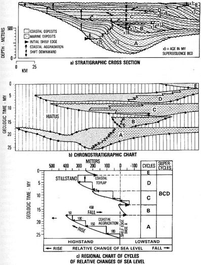
This image shows the three stages involved in the procedure for analysis of a seismic section:
a - seismic section redrawn to show the major reflectors and sequence boundaries
b - chronostratighrapic chart of the same section (the sequence is put in temporal order)
c - graph of relative changes in coastal onlap
(from Vail et al., 1977, in Miall, A.D., 1997, The Geology of Stratigraphic Sequences)
As you can see, sequence stratigraphy grew from the interpretation of seismic stratigraphy.
The original concepts of sequence stratigraphy come directly from the work
of a small research group led by Peter Vail at Exxon Production Research Company.
The basis of sequence stratigraphy rely on seismic, outcrop and subsurface data.
In particular, for what concerns seismic data, the following fact have been deducted:
1 - seismic reflectors are time lines, and not lithological boundaries (this is mostly true in the case of unconformities)
2 - unconformities can be correlated with conformities (that is, the unconformity disappears)
when we are moving from the edge of a basin towards its center
3 - the sequences thus defined by the unconformities consist in lenticular units up to hundreds of meters thick and tens of kilometers wide
| |
| Cyclostratigraphy | Last Updated • May 17, 2016 | |
A wide variety of sedimentary cycles has been identified in the sedimentary record.
All these cycles seem to reflect regularly repeating environmental conditions that can influence sedimentation patterns
(for instance, tides, El Niño events, solar spots, lunar cycles, astronomical cycles, etc.).
While some of these cycles, reflected in the rock record, can be locally important for correlation,
it is only those cycles driven by global climate change that are the most significant in stratigraphical correlation.
Cyclostratigraphy is a branch of stratigraphy that deals with this kind of cycles
the identification of their frequency, and their use in geochronology and chronostratigraphy.
Astronomical cycles of regular frequency occur on time scales
from tens to hundred of thousand years, and possibly up to a few million years in duration.
These cycles are produced by relatively regular variations in Earth's orbit around the Sun,
and are called Milankovitch cycles by the name of the scientist who first recognized them.
These astronomical cycles are responsible for climate change on Earth
by altering the amount of solar radiation oour planet receives from its star.
The identification of these cycles allowed geologists to develop
a finely tuned chronostratigraphic and geochronologic time scale.
Cyclostratigraphy also studies how orbital change affects Earth's climate, oceans and ice-caps
and tries to interpret how the cycles seen in the stratigraphical record have formed.
A brief history
Croll was the first, in 1875, to suggest that orbital variations might influence sedimentation.
Gilbert was the first, in 1895, to discuss a geochronology based on sedimentary cycles.
But it was the Serbian scientist Milutin Milankovitch that, in 1941, showed with numbers
how the solar radiation changed as a consequence of different positions of Earth's orbit in time.
Milankovitch maintained that these changes were responsible for the coming and going of ice ages on Earth.
As in the case of Wegener, Milankovitch's work was originally discarded because
the variations in solar energy he had calculated seemed insufficient to cause glaciations.
It was only in the 1970s that proof of his theory became evident in the sedimentary and stratigraphic record.
The orbital (Milankovitch) cycles
Milankovitch cycles represent only a few of the astronomical cycles that affect our planet.
They are caused by the complex patterns of gravitational attraction between Earth, Moon, Sun and other planets.
These changing patterns influence how much solar radiation reaches Earth, and the times at which it does so
(patterns of insolation and its seasonality).
The three main cycles that have been identified are:
- ECCENTRICITY of Earth's orbit
Earth's orbit shape varies between two extremes: from almost circular (minimum eccentricity) to elliptical (maximum eccentricity). The most important periodicities of eccentricity are at around 100 thousand years (represented by two modes of cycles at 95/104 thousand years) and 404 thousand years.
- OBLIQUITY of Earth's axis
The axis of Earth changes its angle of tilt between 21.5° and 24.5° with a periodicity of approximately 41 thousand years.
This change affects the intensity of the season and the latitudinal distribution of solar radiation, and it mostly affects high latitudes.
- PRECESSION of the equinoxes
Combined with the movement of perihelion (the time at which the Sun is closest to Earth), its frequency is about 20 thousand years, with two modes at 19 and 23 thousand years. Precession affects the timing of the seasons (when the seasons change). That is why we have to have a leap year every four: without this adjustment, in 10,000 years we would have spring in September instead of March in the northern Hemisphere, and vice versa. Modulated by eccentricity, precession is very important at low latitudes.
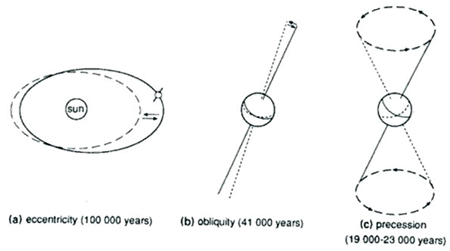
A simple representation of the astronomical variables influencing the climate on Earth
Modified from de Boer, P.L., and Smith, D.G., 1994. Orbital forcing and cyclic sequences, Spec. Publs Int. Ass. Sediment., vol. 19, p. 1-14
How do we identify Milankovicth cycles in stratigraphic record?
- Counting the cycles
The easiest approach is to simply count the cycles, whether in an outcrop, in a core, in geophysical logs, or using other proxies.
- Time-series analysis
Milankovitch cycles can also be identified statistically, through the use of Fourier analysis, which allows to identify a dominant frequency out of a curve built by the sum of several different ones.
- Cycle ratios (precession-eccentricity syndrome)
Since the ratio between Eccentricity, Obliquity, and Precession is approximately 20:5:2:1 (400:100:40:20 thousand years), we look for these patterns in our sequences.
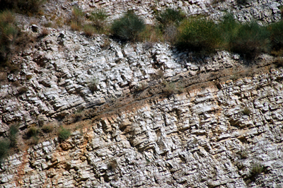
An image of very cyclic (rhythmic) pelagic sedimentary sequence.
White layers are Maiolica Formation limestones, the black layer is the Bonarelly level
or global oceanic anoxic event 1 (OAE 1).
Thickness of OAE 1 is about 1 meter.
Contessa quarry, Gubbio, Perugia, Italy (photo: Alessandro Grippo)
How are the Milankovitch cycles expressed in the stratigraphic record?
A change in climate can effect the physical and biological environment in several different ways.
- Productivity and dilution cycles
A reduction in productivity in ocean waters can cause a decrease in the amount of phytoplankton and zooplankton. Their cyclic disappearance, or dilution within sediments of different kind, can cause Milankovitch cyclicity in the record.
- Redox cycles
Changing amount of oxygen in ocean waters can affect the coloration of rocks, from red (abundance of oxygen), to drab or white (normal conditions) to black (lack of oxygen). The variation of the amount of oxygen can be absolute (a changing ocean circulation) or simply brought on by a changing water depth caused by a sea-level variation. This would simply move the minimum oxygen depth from one location to another.
- Dissolution cycles
Changing chemical conditions can dissolve some carbonates, leaving evidence of dissolution.
How do we correlate the Milankovitch orbital cycles to cyclochronology?
There are different lines of evidence for Milankovicth cycles that can be used to track climate change:
- Ice cores
Mostly, isotopic studies
- Pleistocene and Pliocene
Mostly, isotopic studies and direct evidence from glacial/intergalcial sediments
- Cenozoic and Mesozoic
Mostly, mathematical analysis of sediment cyclicity
Go to part 1 | Go to part 2 | Go to part 3 | Go to part 4 | Go to part 5 | Go to part 6 | Go to the Images Page | Go to the Home Page
© Alessandro Grippo, 2008-2016
| | |